
Gradient Descent
What is Gradient Descent?
Gradient descent is a process by which machine learning models tune parameters to produce optimal values. Many algorithms use gradient descent because they need to converge upon a parameter value that produces the least error for a certain task. These parameter values are then used to make future predictions.
Univariate Gradient Descent
Important Terms/Symbols
For the purpose of this section, we’re going to assume that a simple linear regression model is using gradient descent to fine tune two parameters: b_0 (the y-intercept) and b_1 (the slope of the line). Simple linear regression uses the Mean Squared Error Cost Function, whose equation is shown below.

J(b_0, b_1) represents the cost, or the average degree of error, of the model’s predicted values in comparison to those of the training dataset. To learn more about simple linear regression and the mean squared error cost function, I highly recommend checking out my article.
Visualization
Let’s start by trying to conceptualize what the gradient descent formula does.
Suppose there was a blind man who wanted to get down a hill. How would he go by doing this? He would try and feel his way down the hill by taking the steepest route. Eventually, this would lead to him getting to the bottom of the hill.

This is essentially what gradient descent aims to do—it tries to find its way down a cost graph.
In fact, if we graph the cost in correlation with the chosen values for b_0 and b_1, we end up with a shape similar to that of a valley—a bowl shape.
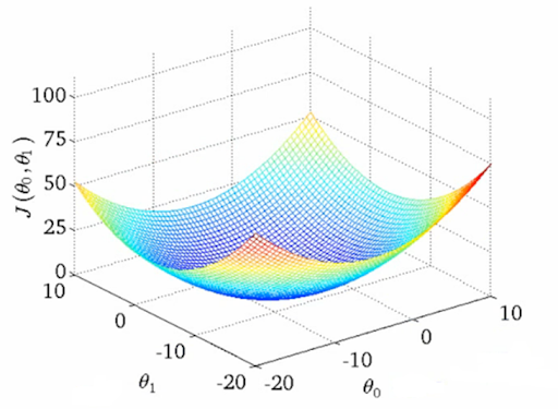
Cost graph including both b_1(theta_1) and b_0(theta_0)
As you can see, this graph looks quite complicated, so let’s focus on the cost graph for each parameter separately.
It’s important to keep in mind that gradient descent actually calculates the cost for both parameters and updates them simultaneously, but we’re just going to focus on one parameter for simplicity’s sake.
If we take a look at the cost graph for a simple linear regression model in relation to just b_0, we’ll see that it looks like a parabola.

b_0 (the y-intercept parameter) in correlation with J(b_0, b_1), the cost
As we can see, we have a simple parabola with a minima at b_0 = 3. This means that 3 is the optimal value for b_0 since it returns the lowest cost.
Keep in mind that our model does not know the minima yet, so it needs to try and find another way of calculating the optimal value for b_0. This is where gradient descent comes into play.
The model will use the gradient descent algorithm to gradually tune the values of b_0 and b_1.
To start this process, our model will initialize all parameters to 0. According to the sample cost graph above, this means that our initial cost is 7.

When b_0 is 0, the cost is 7
So how does gradient descent work to minimize this cost?
It takes the derivative of the cost function, and uses the derivative to figure out how much it should add to or subtract from b_0.
The derivative of the cost function returns the “slope” of the graph at a certain point.
To visualize the slope, we can draw a line that is tangent to the parabola at the point (0, 7). 0 represents the value of b_0, and 7 represents the current cost.

Slope of the graph at (0, 7)
The model multiplies this slope by the learning rate (which we will talk about more later) and subtracts this product from the current value of b_0.
Since the slope is negative, the value of b_0 will become greater, and thus, closer to the optimal value. Let’s take a look at how this works in the graph below:

As we can see, the value of b_0 changed from 0 to 5! This means that we are closer to the optimal value of 3.
The algorithm will now take the derivative of the cost function when b_0 is 5, and carry out the same process as before. This time, however, the slope is positive, so the value of b_0 will decrease. Also take note of how the slope is less steep; this means that our algorithm will take a smaller “step” down the cost graph.

This process will continue until the derivative returns a slope that is very close to 0, signifying that the model has reached a near-optimal value for the parameter being tuned.

The Math
Great! Now we have a general idea of how gradient descent works to optimize parameters. But, we have to remember that the model doesn’t work with each variable one at a time. It makes the calculations for each variable and updates them at once.
To do this, gradient descent actually partial derivatives to find the relationship between the cost and a single parameter value in the equation.
If you don’t know what those are, don’t worry—it’s not necessary to know how to calculate for partial derivatives to understand linear regression.
However, I still recommend watching this Khan Academy video on partial derivatives just so you can get a better understanding of what the gradient descent algorithm is really doing.
Now let’s talk about the gradient descent formula and how it actually works.

Gradient Descent Formula
Let’s start discussing this formula by making a list of all the variables and what they signify.
b_0: As we know, this is one of the parameters our model is trying to optimize. b_0 is the y-intercept of our line of best fit.
b_1: Another one of the parameters our model is trying to learn. b_1 is the slope of the line of best fit.
𝛂: This signifies the learning rate of our algorithm. It is a constant value inputted by the user (i.e 0.1).
It is important not to select a learning rate that is too small, as the algorithm will take too long to converge (reach the optimal parameter values).
A learning rate that is too large, on the other hand, may lead to divergence, where the algorithm gets further and further from the optimal value.
𝜕: Signifies a partial derivative.
J(b_0, b_1): The result from our cost function (the cost divided by 2).
The “:=” represents assignment, not equality. The values of b_0 and b_1 are reassigned every iteration of our algorithm.
Once again, we will use an example to walk through each iteration of this algorithm.
The algorithm will take the partial derivative of the cost function in respect to either b_0 or b_1. The partial derivative tells us how the cost changes in correlation with the parameter being tuned.
If we take the partial derivative of the cost function with respect to b_0, we get an expression like this:

If we take the partial derivative of the cost function with respect to b_1, however, we end up with:

Now, we simply plug these back in into the original gradient descent formula to get:

Now, all we have to do is plug in the values of b_0/b_1, 𝛂, y-hat, and y into each of these equations to tune our parameters.
Let’s say that
𝛂 (learning rate) is 0.1
b_0 and b_1 are initialized to 0
The partial derivative in respect to b_0 simplifies to 20
The partial derivative in respect to b_1 simplifies to -4
If we plug these values into the formulas above, we will get something like this:

Which can be simplified to:

The same process will be repeated over and over again until the values of b_0 and b_1 converge to an optimal value.
After the model converges on these parameter values, it can be used to make future predictions!
But what if there is more than one independent variable?
This is where multivariate gradient descent comes into play.
Multivariate Gradient Descent
Important Terms/Symbols
To learn about multivariate gradient descent, we’re going to assume that we are training a multiple linear regression model. Much like with our example for univariate gradient descent, we’re going to be using the mean squared error cost function. This time, however, the cost function looks a little bit different:

Mean Squared Error Cost Function (multivariate)
The right-hand side of the formula looks exactly the same, but you’ll notice that the left side is expanded to include an n amount of parameters. This is because we need to account for the fact that there could be any number of independent variables. However, the expression still means the same thing: J(b_0, b_1, b_n) signifies the cost, or average degree of error. For more information on this and multiple linear regression, please check out this article.
Visualization
Fortunately, multivariate gradient descent is not that much different from univariate gradient descent. In fact, both algorithms work to achieve the exact same thing in the exact same way. The only difference is that multivariate gradient descent works with n independent variables instead of just one.
To quickly recap, let’s take a look at the cost graph in relation to a single parameter value.

Cost graph in relation to b_0
As you can see, it is able to work its way down the graph to converge upon an optimal parameter value (marked in green). We’ve already covered all of this in the first half of the article, so let’s get right to the mathematics behind multivariate gradient descent.
The Math
Since we already have an idea of what the gradient descent formula does, let’s dive right into it. Like before, the algorithm will update the parameter values by taking the partial derivative of the cost function with respect to the parameter being tuned. Let’s take a look at the formula for multivariate gradient descent.

Multivariate gradient descent
As we can see, the formula looks almost exactly the same as the one for univariate gradient descent. The only difference is that the second equation has been expanded to include all the parameter values other than b_0. This is because b_0 is the y-intercept, while b_1 - b_n are the coefficients of the independent variables. Thus, we have two different equations to encompass each of these two categories.
Just like before, we can take the partial derivative of the cost function with respect to the parameter being tuned. The derivative simplifies to this:

Derivative of cost function + gradient descent formula
As you can see, the derivative with respect to b_0 is exactly the same. The derivative for b_1, however, has one small change.
There is a superscript for the independent variable x. This signifies that the independent variable used depends on which parameter value is being tuned. For example, if the b_2 is being tuned, then the second independent variable’s value is held in x. This makes sense because b_2 is the coefficient of the second independent variable.
To see how this formula works in action, let’s use an example. Let’s assume that we are tuning an equation in the form

As we can see, there are two independent variables (x_1 and x_2) and three parameters to be tuned (b_0, b_1 and b_2). Let’s say we have a multiple linear regression model that has just started the process of gradient descent. This means that all the parameter values are initialized to 0. Let’s also say that:
The learning rate is 0.1
The partial derivative in respect to b_0 simplifies to 10
The partial derivative in respect to b_1 simplifies to 12
The partial derivative in respect to b_2 simplifies to 13
These values are usually computed, but for the sake of simplicity, we have just assumed the values above. Now all we have to do is plug these values into the formula for gradient descent.

As you can see, several substitutions were made into the original formula:
10 plugged in for the partial derivative in respect to b_0
12 plugged in for the partial derivative in respect to b_1
13 plugged in for the partial derivative in respect to b_2
0’s plugged in for b_0, b_1, and b_2
0.1 plugged in for 𝛂
The resulting expressions can be simplified even further to result in the new parameter values for the first iteration of the dataset.

This is the first iteration of gradient descent over the dataset. This process will be repeated hundreds of times until the parameters stop changing by values greater than a certain threshold. For example, if our threshold value is 0.001, and our parameters change 0.00005 from the previous iteration, gradient descent will assume convergence and the “optimal” parameter values will be reached.
We’re done learning with gradient descent! Keep in mind that gradient descent is used by a multitude of models, not just simple and multiple linear regression.
If you liked this article please be sure to check out my next tutorial on polynomial regression. As always, feel free to leave any feedback you have for me in the comments!