
Market Basket Analysis
Project Description
This project will cover associate rule learning, which is a way of extracting correlations in data; more specifically, we’re going to be determining what items in a supermarket are likely to be bought with each other.
For example, our algorithm might determine that salt is often purchased with pepper or that cereal is often bought with milk. This type of algorithm can be used by store owners to determine the placement of items—groceries that are often bought together should probably be placed together.
After our algorithm trains, it should return a list of rules that consist of two-item long relations (i.e., milk is often bought with cereal).
Dataset Analysis
This model, unlike many of the previous ones we have created, is unsupervised. This means that it tries to find relationships within data without labels.
Since we are creating an association rule learning model, our dataset will consist of lists of groceries bought together. Let’s take a look at a sample of the dataset below.
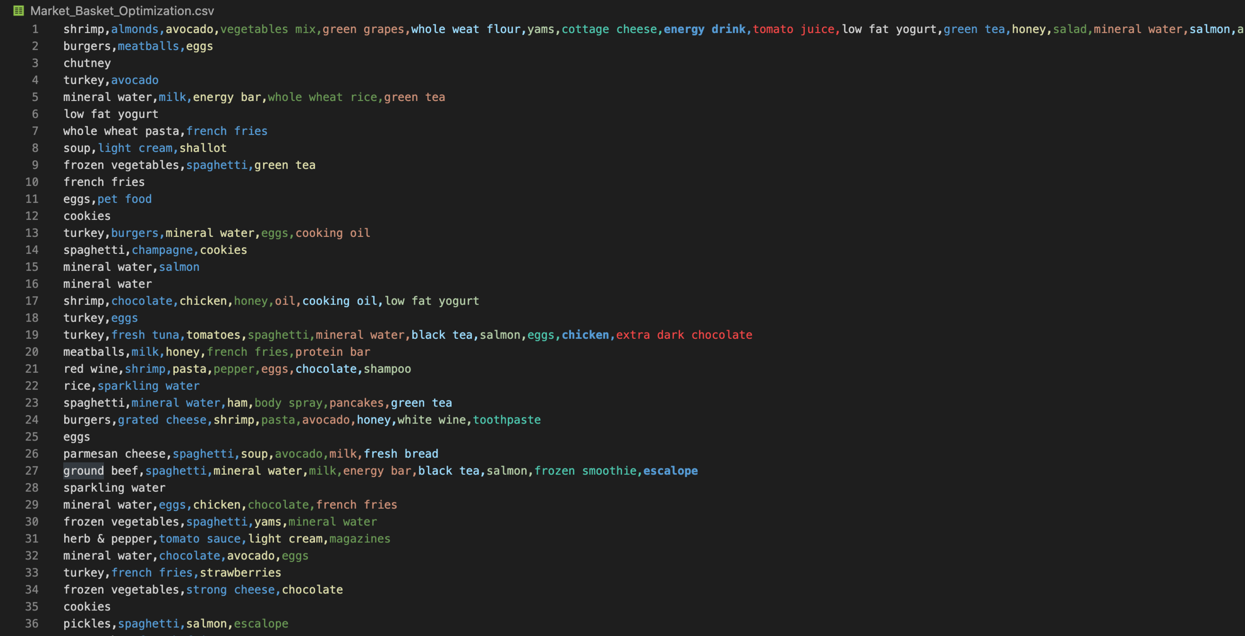
Sample of the dataset
As we can see, the data is contained in a .csv (comma-separated values) file, which means that each item is separated by a comma. Each line contains a list of groceries that a customer bought together.
What’s important to note here is the size of the dataset: we have 7,501 lines, which is a suitable amount of data for association rule learning.
We’ll see that this is an unedited dataset because there are certain lines with only one item. Although these lines won’t help our algorithm identify patterns more efficiently, we’ll keep them to maintain the integrity of the dataset.
Before we move on to importing this dataset, we’ll have to install all the necessary libraries.
Library Installation
For this project, we’ll need to install the following libraries using Pip, Python’s default package management system: Apyori, Pandas, and Numpy.
Apyori is a machine learning library that contains the Apriori associate rule learning model. We will be using this model to analyze our data.
Pandas is a Python library that helps in data manipulation and analysis, and it offers data structures that are needed in machine learning.
Numpy is another library that makes it easy to work with arrays. It provides several unique functions that will help in data preprocessing.
Fortunately, these libraries can be quickly installed by using Pip, Python’s default package management system. All we have to do is enter the following lines of code into the terminal:
pip3 install apyori
pip3 install numpy
pip3 install pandas
Now we can begin coding!
Data Preprocessing
For this dataset, fortunately, we won’t have to do extensive data preprocessing. The Apriori model that we will be using requires the input parameter, transactions, to be a nested list. Because of this, we need to import our dataset as a Pandas dataframe and then convert it to a list using special methods.
To start, we can import Numpy and Pandas as shown below.
import numpy as np
import pandas as pd
Now, we can import the dataset using the .read_csv function that Pandas provides.
dataset = pd.read_csv('Market_Basket_Optimization.csv', header=None)You may notice that we passed in the header keyword argument and set it equal to None. This lets the function know that the first line of the .csv file does not contain column headers, but actual data that needs to be analyzed.
After running the code, a Pandas dataframe containing the data in the .csv file is store in the variable dataset.
However, we must remember that our algorithm requires a nested list as input. Fortunately, we can transform our dataframe into a list with the following line of code:
dataset = dataset.values.astype(str).tolist()
In the above line of code, we take in the values in the dataframe by using the values method and ensure that they are all of type String. Then, we move these values into a list by using the tolist method. The variable dataset now holds a nested list, not a Pandas dataframe.
If you were to print out the entire list (which is quite long), you will notice that there are a lot of ‘nan’ values that were not present in the original data.
This is because each line in the original csv file was not of the same length; thus, when Panda read the csv file column by column, there were several blank places. These spaces are represented with the string ‘nan.’
After running this line of code, we have successfully completed the data preprocessing portion. Now we can create our model using Apyori.
Model Creation
The implementation of the associate rule learning algorithm is quite simple—since apriori is a function that returns a list of rules, we merely have to instantiate a variable to hold the rules and pass in the required arguments. Before we do this, however, it’s important to briefly go over these parameters as understanding them is essential to associate rule learning.
transactions is the argument through which you pass in the input data
min_support is the minimum level of support required for a possible itemset. Support, in simple terms, signifies how frequently a certain itemset appears in a dataset
min_confidence is the minimum level of confidence required for a possible itemset. Confidence indicates how often a certain rule, or relationship, was found to be true.
min_lift is the minimum level of lift required for a possible itemset. The concept of lift is slightly more abstract: we don’t need to delve too far into this argument for the scope of this article. I will, however, be publishing another article dedicated to explaining associate rule learning, so make sure to look out for that.
max_length is the maximum length of an itemset (rule)
min_length, as you’ve probably guessed, is the minimum length of an itemset (rule)
random_state is a parameter that passes in a random seed to the algorithm. This ensures that your model creates the same rules each time it runs on a certain dataset. Although not required, this argument is helpful when following along with a tutorial.
With this information in mind, let’s create our and get the list of rules. We can do this as shown below:
from apyori import apriori
rules = apriori(transactions=dataset, min_support=.005, min_confidence=.25, min_lift=2.7, min_length=2, max_length=2, random_state=0)
results = list(rules)
The above code passes in values for each of the parameters discussed previously. I spent some time tuning these parameter values so that we would get a suitable number of rules. Feel free to experiment with these parameters yourself, as it can be a great learning experience!
In the last line above, we simply create a new variable, results, which contains the data in rules in a list form.
We do this so that we can extract all the important information using list indexing in the next section.
Result Processing
In this project, we will need to process the data in a way that is easily readable. For this, we will need to first go over the output of the apriori function that we used.
Our algorithm will return a list containing lists. Each inner-level list will contain the following structure:
frozenset({‘item1’, ‘item2’})
support
OrderedStatistic[items_base=frozenset(‘item’), items_add=frozenset(‘item’), confidence, lift]
This structure will make much more sense once we actually begin indexing the items.
First, we’ll need to extract the base items and the added items from our rule sets. As we can see above, these items are stored in frozenset(). In order to index this, then, we’ll have to convert it to a list.
Let’s do this using list comprehension as shown below.
base_item = [list(result[0])[0] for result in results]
added_item = [list(result[0])[1] for result in results]
Now, we can index the support, which is the first item in each result.
support = [result[1] for result in results]
Finally, we can begin to index the confidence and lift. If we take a look at the output structure above, we’ll see that we have to index into the third and fourth items in OrderedStatistic, which is located in a list at the second index point. Let’s extract these elements as shown below.
confidence = [result[2][0][2] for result in results]
lift = [result[2][0][3] for result in results]
Finally, we can put all these variables together using Python’s zip function.
final_results = list(zip(base_item, added_item, support, confidence, lift))
Now all of our results are placed into a clean list that can be printed out; however, it might be even easier to place all of these items into a Pandas dataframe.
This can be done by using Pandas’s dataframe function.
organized_results = pd.DataFrame(final_results, columns=['Base Item', 'Added Item', 'Support', 'Confidence', 'Lift'])
organized_results.to_csv('results.csv')
We store the dataframe in organized_results and then save it in a csv file in the second line of code. Now, we can view all our results in a clean data table by opening up the csv file. This can be done using any application, but I’m using the csv extension on VSCode to preview the csv in a clean manner.
Let’s take a look at the results in the image below:
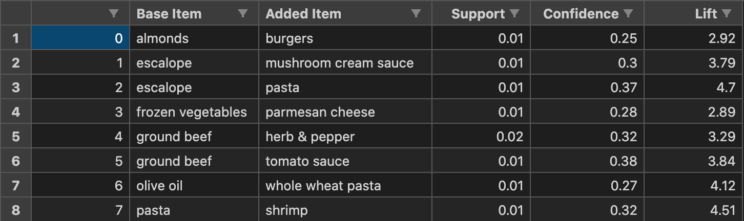
As we can see, our algorithm returned 8 sets of rules. These items can be organized in whatever manner you choose. On VSCode, you can choose to rank the items based on whichever column you want. In the above column, we rank the items based on the alphabet in the base item column. In each row, we can see a base item and an added item as well as the corresponding statistics for that rule.
As discussed before, these rules can be used by store managers to determine the placement and the method of promotion for groceries.
Conclusion
In this project, we covered the use of the apriori algorithm to complete the classic market basket analysis associate rule learning problem.
It’s important to know, however, that such algorithms can be used for a variety of tasks. It can be used in anomaly detection, in which the algorithm identifies transactions or events that do not fit in with any rule in the ruleset. It can also be used in recommender-systems: many streaming services such as Netflix use an advanced version of the algorithm discussed to recommend movies and television shows to their audience.
Once again, although this was a very simple example of associate rule learning, it does provide a strong foundation for one to delve into more complex models and algorithms.
I hope this article was helpful and entertaining. If you have any feedback, please feel free to leave a comment! Stay tuned for my next tutorials and projects on machine learning!