Wildfire Detection

Project Description

Every year, California experiences instances of large-scale wildfire detection due to blazing summer heat. These wildfires can cost state governments up to 400 billion dollars in just property damage.

But why are wildfires so difficult to stop?

This is because they double in size every 5 minutes, so early detection is a must in order to limit the damage wildfires can cause.

The goal of this project is to create a machine learning model that can detect wildfires via computer vision. Our model will need to output one of two values signifying whether the given image is one of a wildfire or not.

• 1 represents a wildfire

• 0 represents no wildfire

Dataset Analysis

This project is one that I decided to pursue by myself, so I had to find a dataset online for my project. Eventually, I came across this great dataset created by Ahmed Saied. t

Note: All the data and code samples for this project can be found in my GitHub Repository.

Let’s take a look at the dataset directory structure now:

From this picture, we see that there is one main data directory which contains two subdirectories called test and train. Each one of these subdirectories contains two additional subdirectories called not_wildfire and wildfire. This means that there are 4 different folders in which our images are stored.

Now let’s break down the number of images in each of these folders:

• Under the train dataset, we have 393 images of wildfires and 459 images of non-wildfires.

• Under the test dataset, we have 101 images of wildfires and 101 images of non-wildfires.

Fortunately, this means that our dataset is balanced (which means that there are similar numbers of samples in each category), and we won’t have to do any additional image augmentation to a specific category in our dataset; we can just perform the same image preprocessing on all categories.

Just for fun, let’s take a quick look at some of the images to see what we’re working with, and then we’ll move on to library installation.

Wildfire (1)

No wildfire (0)

Library Installation

To complete this project, we need to install three important libraries: OpenCV, Tensorflow and Numpy

• OpenCV is a library that will help us take pictures with our computer’s camera. It also provides many resources for machine learning itself, but we’re going to use TensorFlow to create our model.

• Tensorflow is a library that we will be using to create deep learning models such as neural networks. It provides several data preprocessing classes which will help us extract data from images and other input sources.

• Numpy is another library that makes it easy to work with arrays. It provides several unique functions that will help in data preprocessing.

Fortunately, these libraries can be quickly installed by using Pip, Python’s default package-management system. All we have to do is enter the following lines of code into terminal.

pip install numpy
pip install tensorflow

Now we can begin data preprocessing!

Data Preprocessing

Image Augmentation

One of the most important parts of creating a computer vision model is image augmentation, which is the process by which we artificially create images by transforming the given inputs to generate more data and reduce chances of overfitting. Feel free to check out the link above to learn more about this topic.

To get started with image augmentation, we can instantiate Tensorflow’s ImageDataGenerator class, which will help us run a series of transformations on each image.

First, we’ll create an instance of the class for our training data to apply the necessary transformations. This can be done as shown below. First, we import the necessary class, and then we simply create an instance through variable assignment.

from tensorflow.keras.preprocessing.image import ImageDataGenerator
train_datagen = ImageDataGenerator(rescale=1./255, shear_range=.2, vertical_flip=True, horizontal_flip=True, zoom_range=.2)

train = train_datagen.flow_from_directory(directory='data/train', target_size=(128, 128), class_mode='binary')

The .flow_from_directory method extracts all the images from the given folder and places them into a DirectoryIterator, which consists of Numpy arrays in batches.

Now, all we have to do is create a different instance of the class and use the same .flow_from_directory as we did before. However, we don’t perform image augmentation since this is the test data, and we want to simulate a real-life situation as accurately as possible.

test_datagen = ImageDataGenerator(rescale=1./255)
test = test_datagen.flow_from_directory(directory='data/test', target_size=(128, 128), class_mode='binary')

Now we have two DirectoryIterators that contain the train and test images separately. Each of these can be directly inputted into the CNN, as they contain the both the inputs (images) and the outputs (labels).

This is because Tensorflow is able to find the image labels based on the directory structure we set up previously. Since the not_wildfire directory comes before the wildfire directory, non-wildfires correspond with outputs of 0, and wildfires correspond to outputs of 1.

Creating the Network Architecture

An Overview

Convolutional neural networks, the type of model we will be using for this project, can be of different sizes and have different architecture setups. For this project, I tested several different models and found an architecture that trains quickly and works well for wildfire detection.

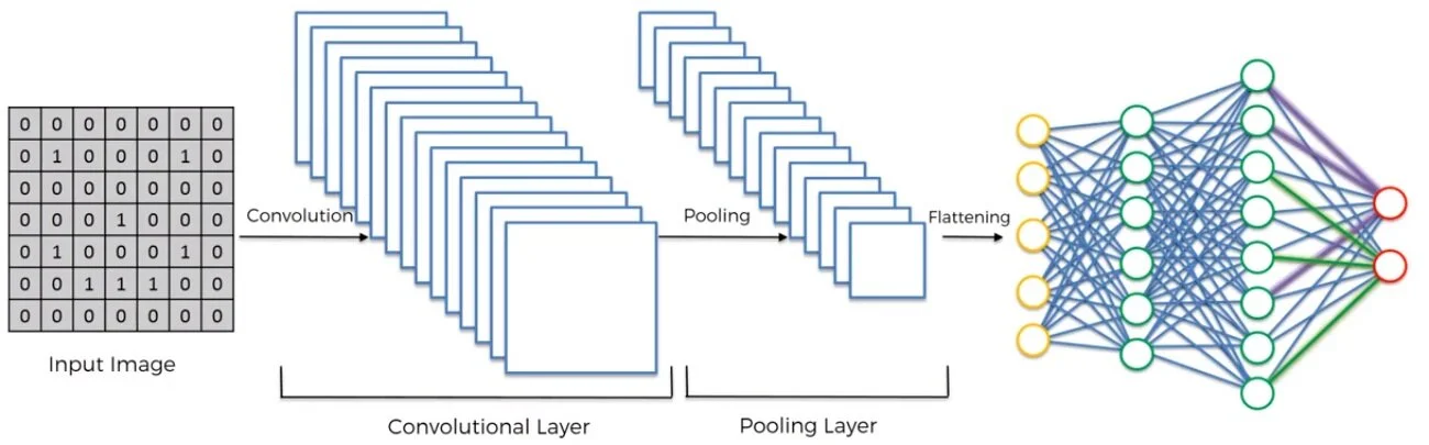
Let’s quickly go over the general structure of a CNN so we know what to build:

1. A convolutional layer will be used to create feature maps (aspects of an image that are of interest to the CNN)

2. This feature map is then inputted into a pooling layer, which condenses the feature map into a smaller array

3. Several convolutional and pooling layers can be used in a network architecture, depending on the image size and/or complexity of the detection problem

4. After the final pooling layer, the input is then flattened, or reshaped into a vector

5. The vector is then inputted into a fully-connected artificial neural network, which delivers the final predicted output

This might be a little difficult to understand at first, so here’s a concise diagram I found from Panadda Kongsilp’s great article on CNN’s.

Let’s move on to implementing the first step of this architecture—the convolutional, pooling, and flattening layers.

Part One

In this section, we’ll work on transforming each image into a vector that can be inputted into a fully-connected network. To do this, we need to first import a variety of classes that we will need. Then, we can begin the convolution + pooling phases.

from tensorflow.keras.models import Sequential
from tensorflow.keras.layers import Dense, Conv2D, MaxPool2D, Flatten

The first statement imports the Sequential class, which is the class used to build sequential neural networks. The next statement imports Dense, Conv2D, MaxPool2D, and Flatten, which are the classes that will help us build each layer of the neural network.

• To build each convolutional layer, we’ll use Conv2D

• To build each pooling layer, we’ll use MaxPool2D

• To flatten all the data, we’ll use Flatten

• Finally, the layers in the ANN can be made by using Dense

To begin building the network, we must instantiate the Sequential class so we can use the .add method to build the network architecture. This can be done as shown below.

cnn = Sequential()

Now we can add the convolution and pooling layers to the network as shown below; the amount of these layers can be changed, but keep in mind that changing the network will cause differences in performance. Thus, it is important to test different network architectures and determine which works best for the problem at hand.

After testing the several different size networks, 3 convolution layers and 2 pooling layers seemed to work the most efficiently on my computer. Let’s work to implement this in code.

cnn.add(Conv2D(filters=32, kernel_size=3, activation='relu', input_shape=[128, 128, 3]))
cnn.add(MaxPool2D(pool_size=2))

cnn.add(Conv2D(filters=32, kernel_size=3, activation='relu'))
cnn.add(Conv2D(filters=32, kernel_size=3, activation='relu'))
cnn.add(MaxPool2D(pool_size=2))

The input_shape argument is only needed in the first layer because that’s the layer where we input the image itself; in the rest of the layers, the input is the output of the previous layer.

Now that we’ve finished the convolution/pooling process, we can just flatten the output from the final pooling layer so that it can be inputted into an ANN.

cnn.add(Flatten())

Great! Now we can move on to the next portion of our network architecture: the fully-connected layer.

Part Two

This can be build by creating an ANN with Dense, much like how we would if this were a regular classification problem. Once again, the number of Dense layers and the nodes in each layer can vary, but the numbers I have selected below created a network with good accuracy and training time.

Let’s implement this part of the network into code so that we can test our image classifier.

cnn.add(Dense(units=128, activation='relu'))
cnn.add(Dense(units=128, activation='relu'))
cnn.add(Dense(units=128, activation='relu'))
cnn.add(Dense(units=128, activation='relu'))
cnn.add(Dense(units=128, activation='relu'))
cnn.add(Dense(units=1, activation='sigmoid'))

As you can see, this code creates an ANN with 4 hidden layers, one input layer, and one output layer. The final layer will output either 0 or 1 depending on the image’s classification.

But since we’ve completed this layer, we’ve completed the architecture of our neural network. Now all we have to do is compile the CNN and then we can begin training it in the next section.

We can now compile the network by using the .compile method of the Sequential class as shown below.

cnn.compile(optimizer='adam', loss='binary_crossentropy', metrics=['accuracy'])

Now we can finally train and test our neural network to see how well it performs.

Training and Testing the Neural Network

This step can be done with only one line of code. The .fit method of the Sequential class has several parameters that we must take a look at. First, we can pass in a value to x, the parameter that takes in the training dataset of images. We have this stored in the variable train.

The next argument we must take a look at is validation_data, which will be used to determine the accuracy of the classifier on separate test data. We have this data stored in the variable test.

The final parameter that we are going to take a look at is epochs, which is the number of dataset iterations our CNN will train for. For this, we are going to input 100, as this number of epochs ensures that our classifier will be well-trained without overfitting (I determined this by testing several different numbers, but you can feel free to experiment yourself as well).

Great! Since we now know the variables that we will input, let’s implement this into code.

cnn.fit(x=train, validation_data=test, epochs=100, batch_size=32)

If we run our program now, we should receive a validation accuracy (denoted by val_accuracy) of around 98 percent.

The final thing that we’re going to do is save our model so that we can use it to classify single images.

Fortunately, this can be done with Sequential’s .save method, which will store the model in its own directory. Let’s go ahead and put this into our code.

cnn.save('model', save_format='tf')

Testing on Single Images

Now that we’re done training and testing our neural network, let’s create another file called test.py in which we create and define a function that will use the neural network to classify single input images as either a wildfire or not a wildfire.

Let’s start by importing all the classes we will need for this section.

from tensorflow.keras.models import load_model
import numpy as np 
from tensorflow.keras.preprocessing.image import load_img
from tensorflow.keras.preprocessing.image import img_to_array

Now, let’s figure out which images we will select from the test dataset to test our network performance on.

Here are the images that I chose:

data/test/not_wildfire/non_fire.205.png

data/test/wildfire/fire.619.png

Since we want to test both of these images, let’s create a variable called image_path that contains the path of the image we want to test.

image_path = 'data/test/not_wildfire/non_fire.205.png'

Now, we can define a function called predict() that takes in the image path and returns an output 1 or 0, depending on the neural network’s classification.

Inside the function, we’re first going to load the model that we saved in cnn.py, and then we are going to load the image and convert it to an array. Let’s do this now:

def predict(image_path):
    cnn = load_model('model')
    image = load_img(f'{image_path}', target_size=(128, 128))
    image = img_to_array(image)

Notice how we use the same image size as we did when training the network. This is necessary as the neural network expects the same size image each time it predicts; if the size is different, the network will throw an error.

There’s just one small technicality we have to deal with before we use the classifier to predict what category the image belongs to. When we trained our network, we created a DirectoryIterator with a column containing the batch each image was in.

Since we’re only testing on a single image, there are no batches; this will cause the classifier to raise an error because of missing dimension. Thus, we add a column containing the integer 1, indicating an arbitrary batch number.

After doing this, we can use the .predict method of our model and input the image we have just transformed. Since neural networks output the probability of the image being a certain category in a double nested array, we can simply index twice into the returned prediction and transform the number into an integer.

def predict(image_path):
    cnn = load_model('model')
    image = load_img(image_path, target_size=(128, 128))
    image = img_to_array(image)
    image = np.expand_dims(image, axis=0)
    prediction = int(cnn.predict(image)[0][0])
    return prediction

Nice! Now we can call the function and assign the return value into a variable called prediction.

prediction = predict(image_path)

Now, although we don’t strictly need to, let’s create a simple if/else statement to make the program print either ‘Wildfire’ or ‘Not a wildfire’ to make it easier for us to read the output.

if prediction == 1:
    print('Wildfire')
elif prediction == 0:
    print('Not a wildfire')

If we run the program, we will receive the output ‘Not a wildfire’, which is exactly what we were expecting. Let’s test the network on the other image that we had selected by changing the image path.

image_path = 'data/test/wildfire/fire.619.png'

This time, we receive the output ‘Wildfire’, which means that our neural network has once again successfully categorized the image!

Taking a Picture and Predicting

We’re just going to do one final thing before we conclude this project. We’re going to create yet another file which will use the predict() function we created to classify an image that the computer camera takes.

Let’s start by importing all the libraries we will be using:

from cv2 import cv2
import time
from test import predict

Now, we will instantiate the VideoCapture class by inputting the camera we want to use (for most people with built-in cameras, this number would be 0).

cam = VideoCapture(0)

Now, we’re going to create an infinite while loop since we want our program to take pictures at specified time intervals. Inside this loop, we’re going to read the current frame of the video and ensure that the frame was properly captured. This can be done as shown below.

while True:
    is_error, img = cam.read()
    if not is_error:
        print('Error when grabbing frame')
        break

The .read method returns a list of which the first index contains a boolean; True signifies that the frame was properly captured, and False indicates that it was not. The second index of the list contains the frame itself.

If there is an error, our program will tell the user that there was an “Error when grabbing frame” and break out of the loop.

Now that we’ve completed this portion, let’s write the image to a file by using OpenCV’s imwrite() function.

while True:
    is_error, img = cam.read()
    if not is_error:
        print('Error when grabbing frame')
        break
    cv2.imwrite('image.png', img)

Finally, we’ll call the predict() function we created and assign its return value to prediction. We’ll then print this prediction and wait for 10 seconds before starting the next iteration of the loop.

while True:
    is_error, img = cam.read()
    if not is_error:
        print('Error when grabbing frame')
        break

    cv2.imwrite('image.png', img)
    prediction = predict('image.png')
    print(prediction)
    time.sleep(10)

Great! If we run our program now, we should see a series of 0’s and 1’s depending on whether our classifier categorized the picture taken as a wildfire or not a wildfire.

You may notice that the network classifies more images incorrectly when you take pictures around your home; this is because it was trained with pictures of nature and the natural environment. Thus, images of a home environment and/or any other non-natural environment will be more foreign to it.

Conclusion

Overview

We were able to create a neural network capable of analyzing images of the natural environment to determine whether or not a wildfire is present. By using Tensorflow’s Sequential model, we were able to receive results of up to 94 percent, which is extremely accurate!

Potential Improvements

As always, there are several ways to improve upon the model that we created. For example, we could:

• Add more data to our dataset so that our model has experience in a variety of environments

• Try larger network architecture setups for deeper image analysis

• Try a different approach to object detection such as image segmentation

Feel free to try out the suggestions and above and let me know in the comments if you were able to achieve better results!

If you liked my article, please make sure to check out some of my other posts for more projects and/or tutorials on machine learning. Make sure to leave any feedback you have for me so that I can improve for my next article. Thanks for reading!